Taking Images
Below are some images used in this project for the image rectification task:
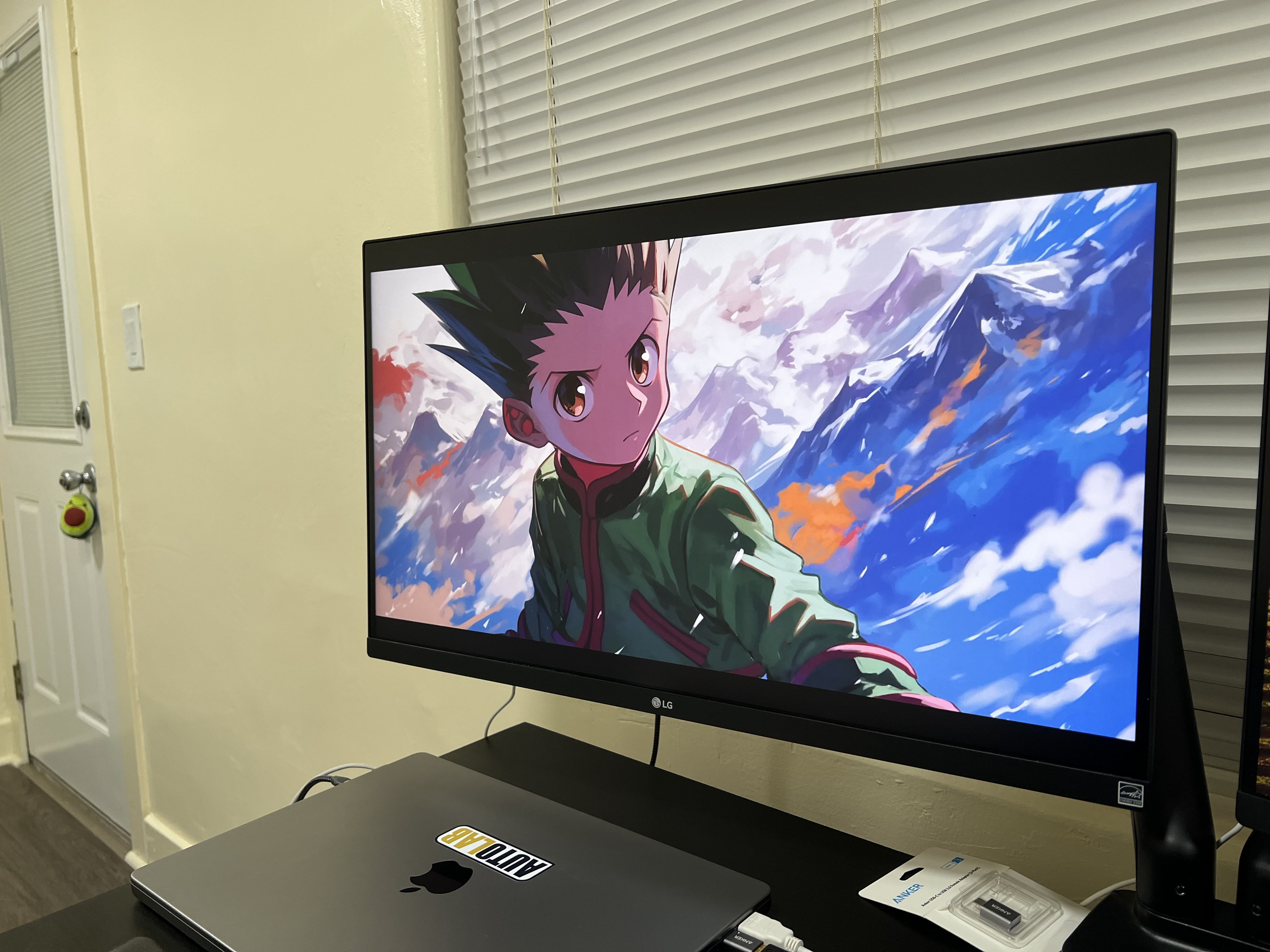
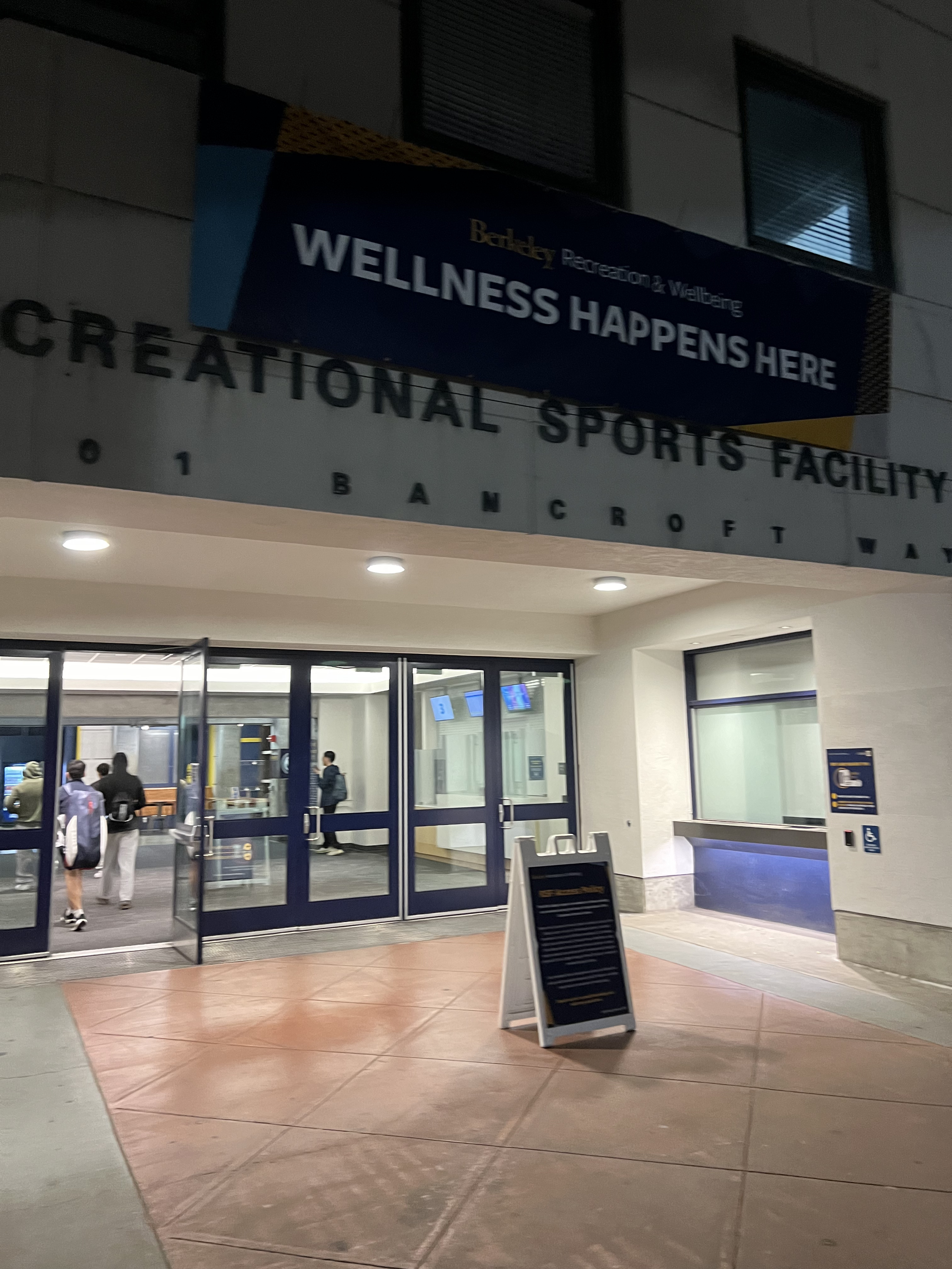
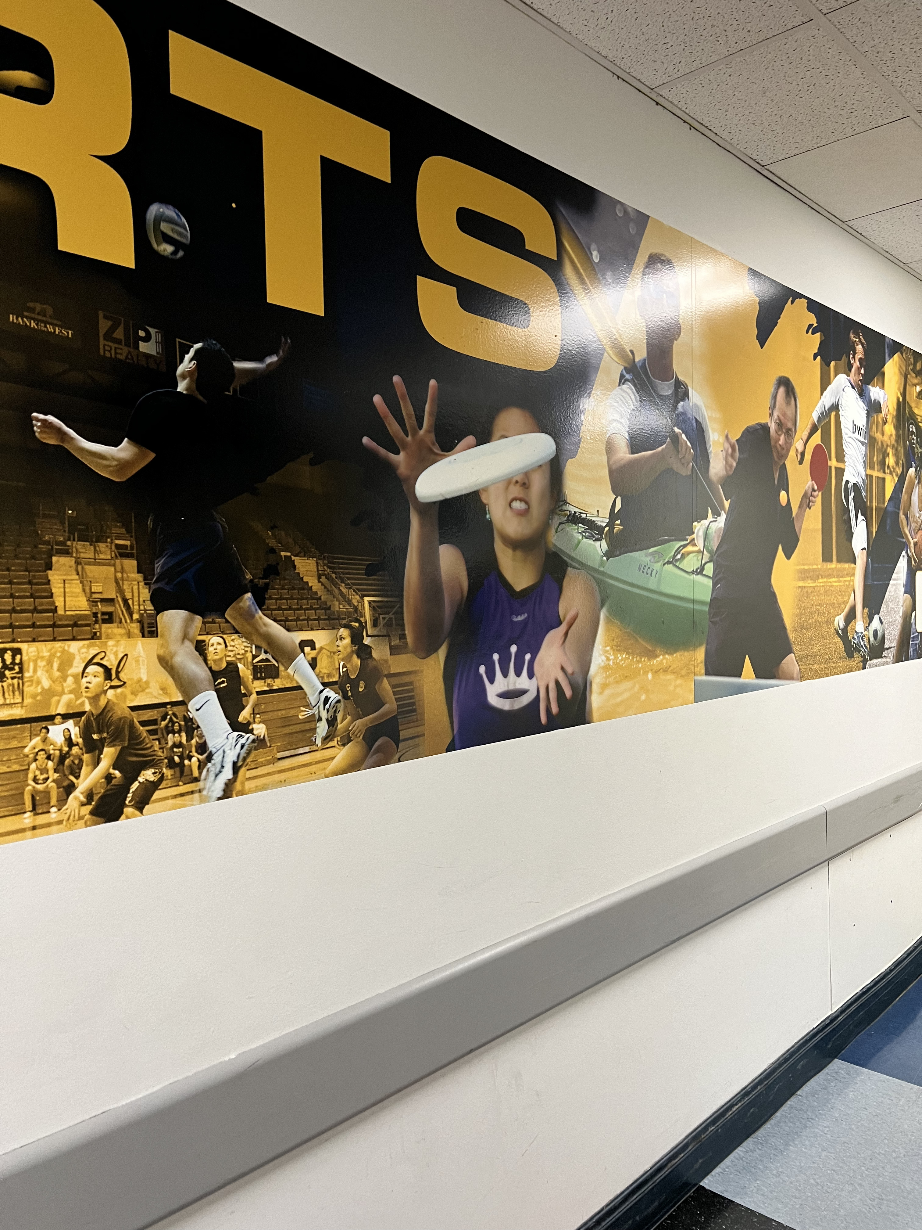
An exploration of image transformation and homography recovery
Below are some images used in this project for the image rectification task:


Before warping images into alignment, we need to recover the parameters of the transformation between each pair of images. In our case, this transformation is a homography, represented by the equation:
Here, H is a 3x3 matrix with 8 degrees of freedom (the lower-right corner is a scaling factor and can be set to 1). We can recover the homography by establishing a set of (p’, p) pairs of corresponding points from two images.
The function structure used for homography recovery:
In this function, im1_pts and im2_pts are n-by-2 matrices holding the (x, y) coordinates of n point correspondences from the two images, and H is the 3x3 homography matrix. Setting up a matrix equation, Ah = b, allows us to solve for the entries in H. This process requires more than 4 points to create an overdetermined system, which can be solved using least-squares to improve stability and accuracy.
We can set up the system of equations as follows (cited from CS180 Project 4B):
Once the coefficients h_i are computed, the homography matrix can be constructed as:
With the homography matrix H, we can compute coordinate warps in homogeneous coordinates by multiplying H with the original coordinates and then scaling:
This results in transformed coordinates:
Now that we know the parameters of the homography, we can use this matrix to warp each image towards a reference image. The function structure for this operation is:
In this process, im is the input image to be warped, and H is the homography matrix. The warping can be done using either forward or inverse mapping. I used inverse mapping to trace the coordinates of the output image back to the original image, applying linear interpolation to fill in the new image plane.
One important aspect is determining the size of the resulting image. I predicted the bounding box coordinates by transforming the four corners of the input image using H.
With the homography and warping code in place, I then tested them all together by performing “rectification” on an image. This essentially just process re-projects an image to make known rectangular objects (like paintings or tiles) appear straightened and aligned. This results below help verify our techniques to ensure we are getting accurate/decent enough estimations.
Once we have estimated the homography matrix, we can use it to re-project one image onto the plane of another for stitching. For instance, to project Image 1 onto Image 2, we perform an inverse warp to achieve a smooth reprojection.
This involves transforming the four corners of Image 1 using the homography matrix to map them onto Image 2, defining the bounding box where the re-projected image will be placed. The next step is to interpolate the pixel values of Image 1 to align accurately within this bounding box. Using scipy.interpolate.RegularGridInterpolator, we interpolate the pixels of Image 1 and place the interpolated values at corresponding locations in the final image.
For cases involving multiple images without direct homographies between each pair, transformations can be calculated by chaining homographies. For example, if there is a homography from Image A to Image B and another from Image B to Image C, the homography from Image A to Image C can be obtained by multiplying the two matrices.
For my examples, I basically just selected the four corners of a rectangular object as points in im1_pts and define im2_pts as a perfect square, such as some scaled version of these coordinates [0, 0; 0, 1; 1, 0; 1, 1].
Results:
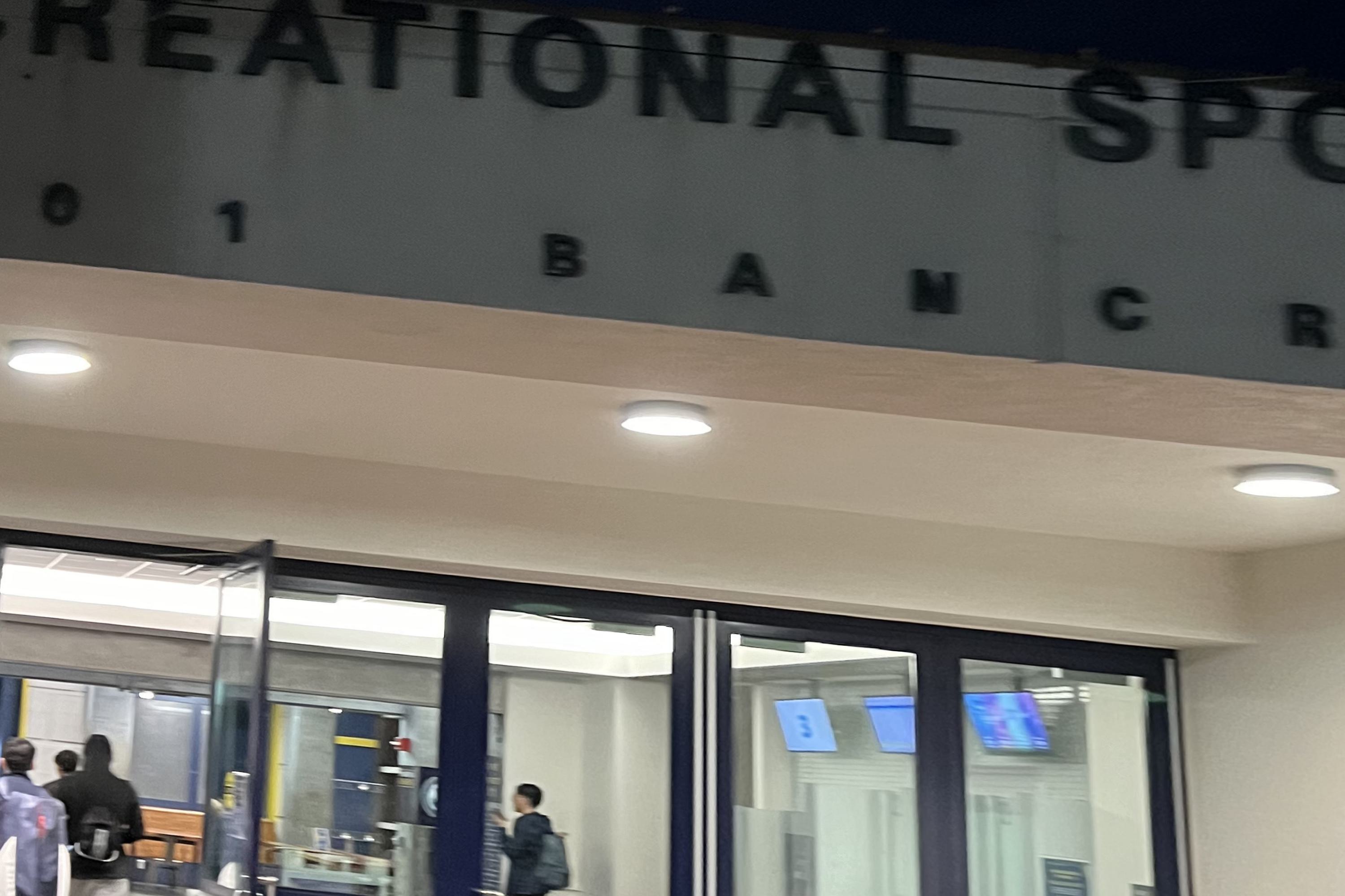
Directory containing rectified images:
To create a seamless mosaic, the images must be registered and blended together. Rather than overlaying one image directly onto another, which can cause strong edge artifacts, a weighted averaging technique is used. I selected one image as the reference and warped the other to align with the reference plane.
Each pixel in the region of an image is assigned a weight based on its Euclidean distance to the nearest edge using a distance transform. This distance is normalized from 0 to 1, serving as a blending weight. For improved results, a 4-level Laplacian pyramid was applied to handle different frequency bands. High-frequency details are blended based on the maximum distance transform values, while low-frequency details are combined using a weighted linear blend.
The following images were used as inputs for the mosaicing process:
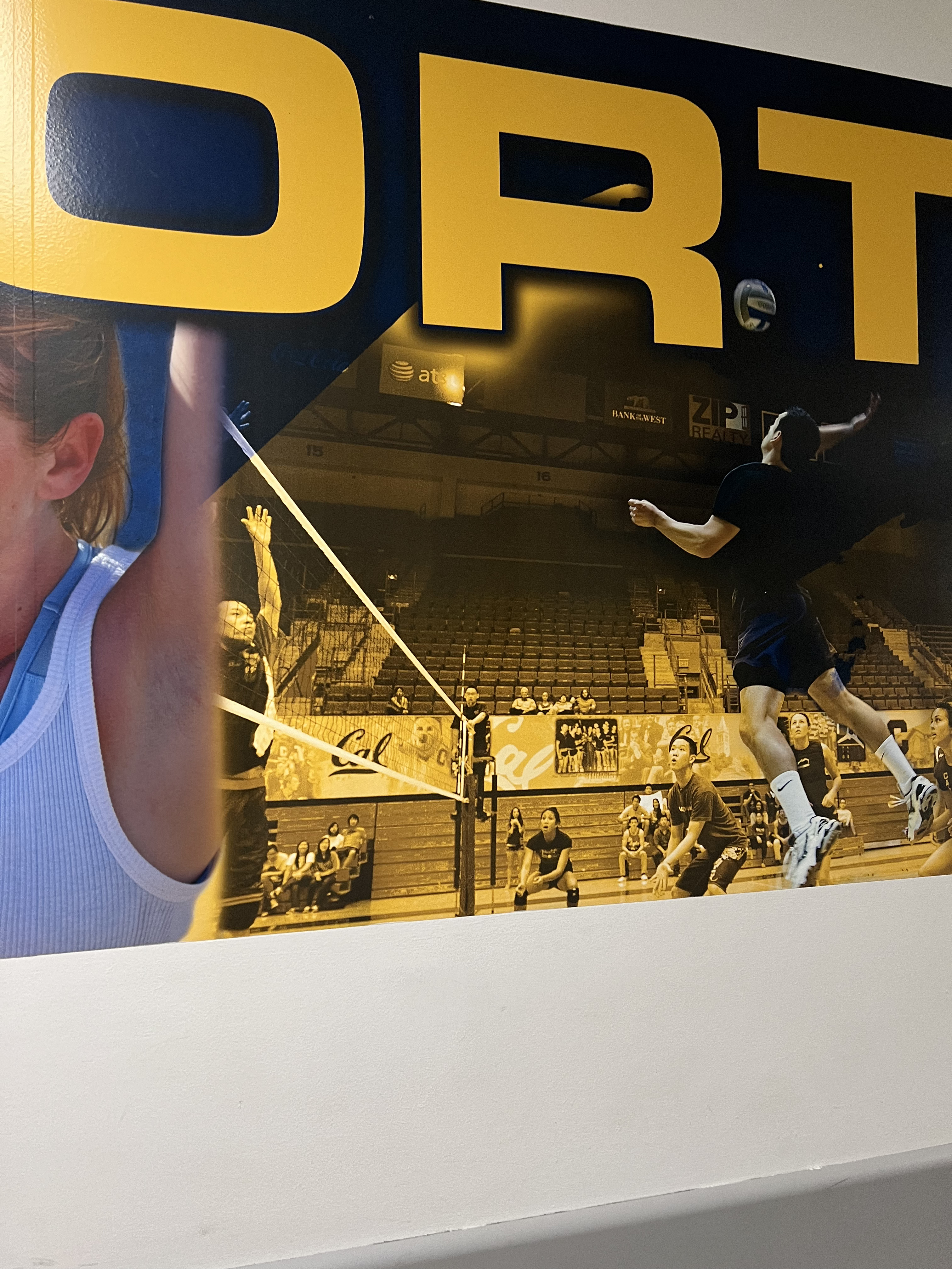
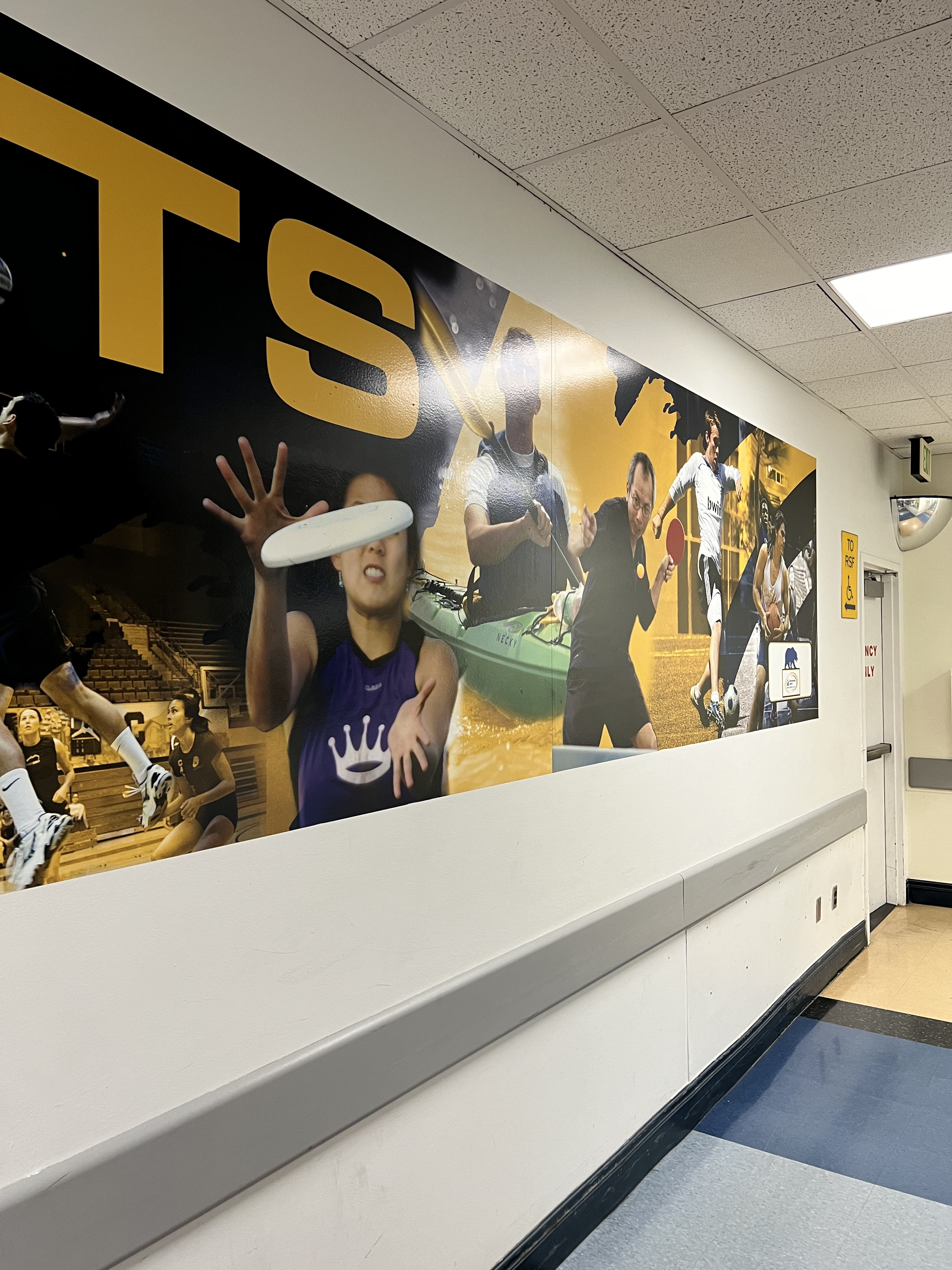
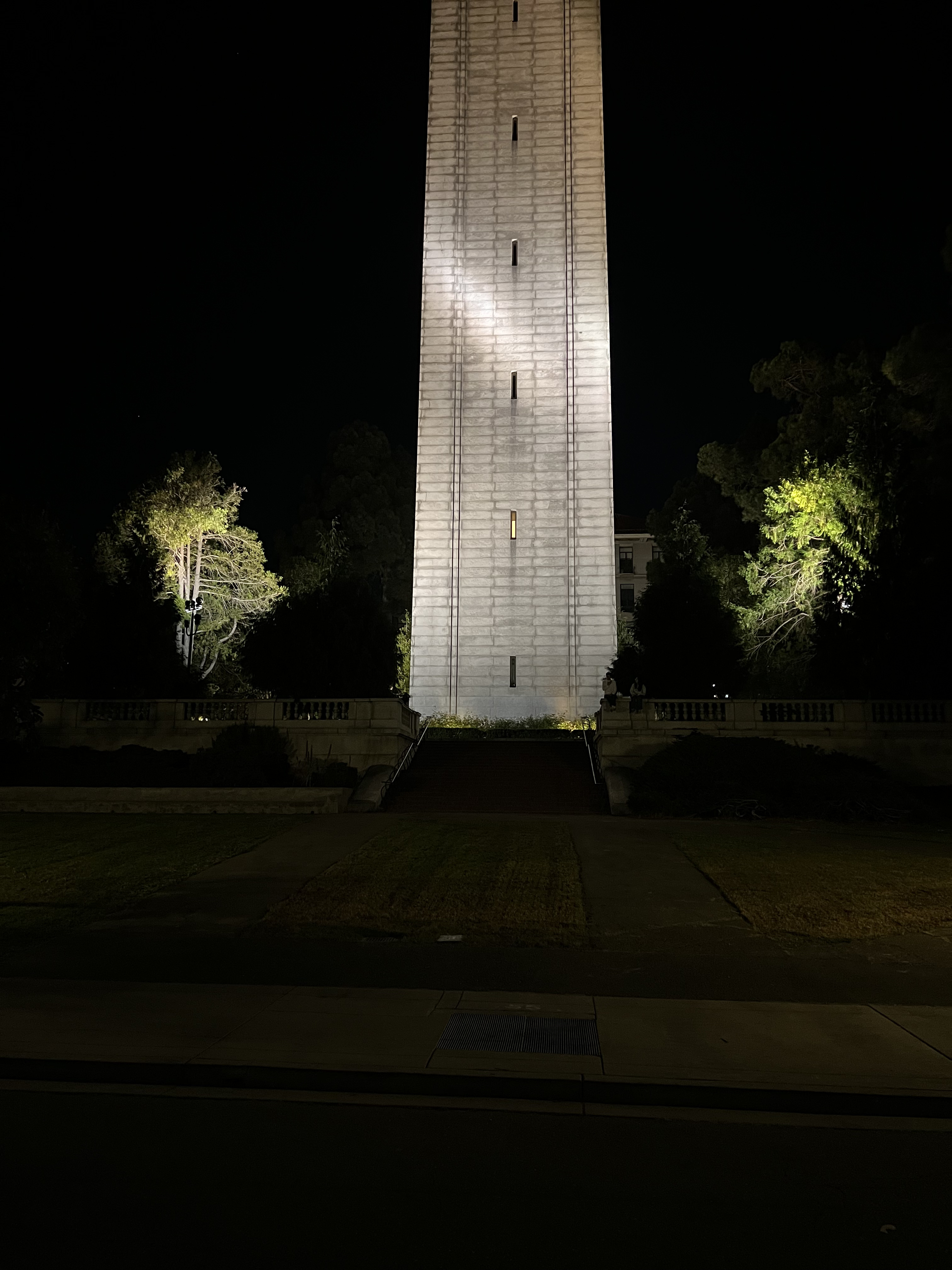
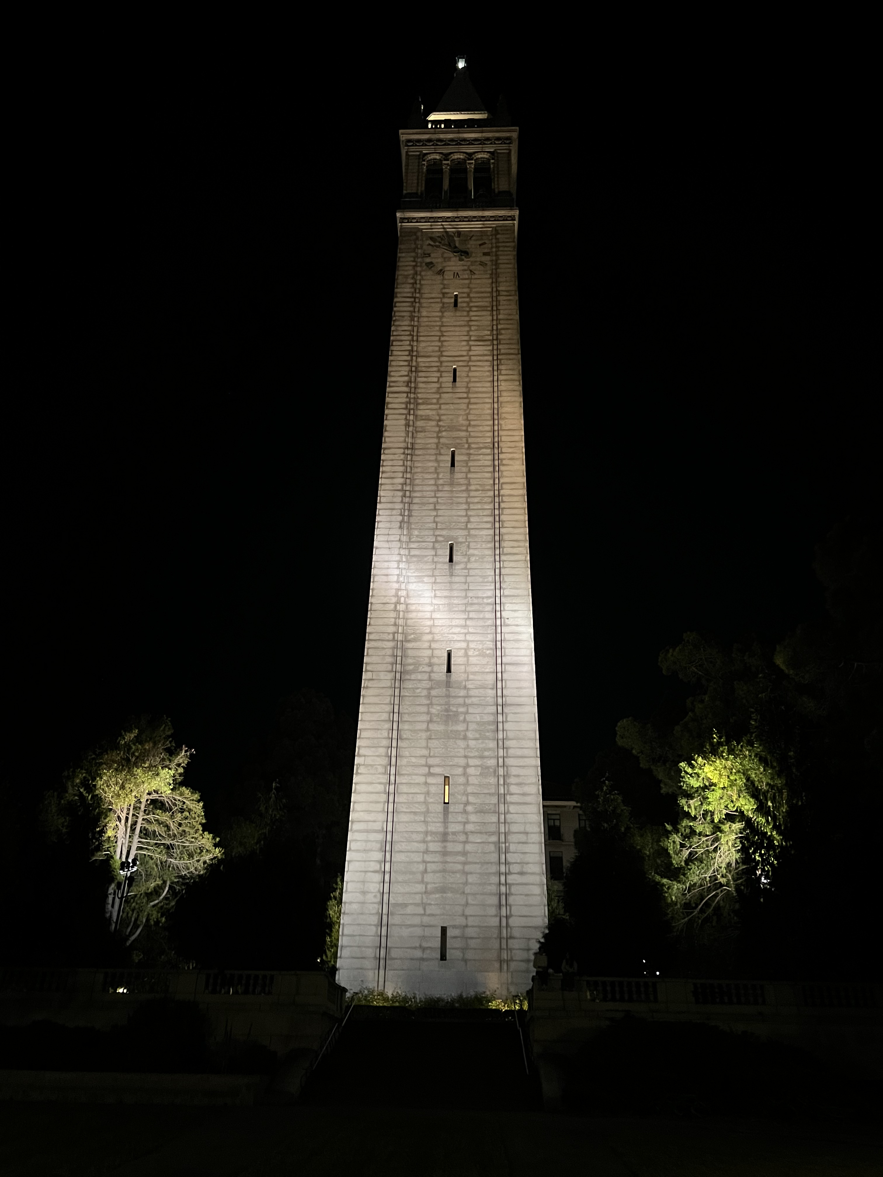
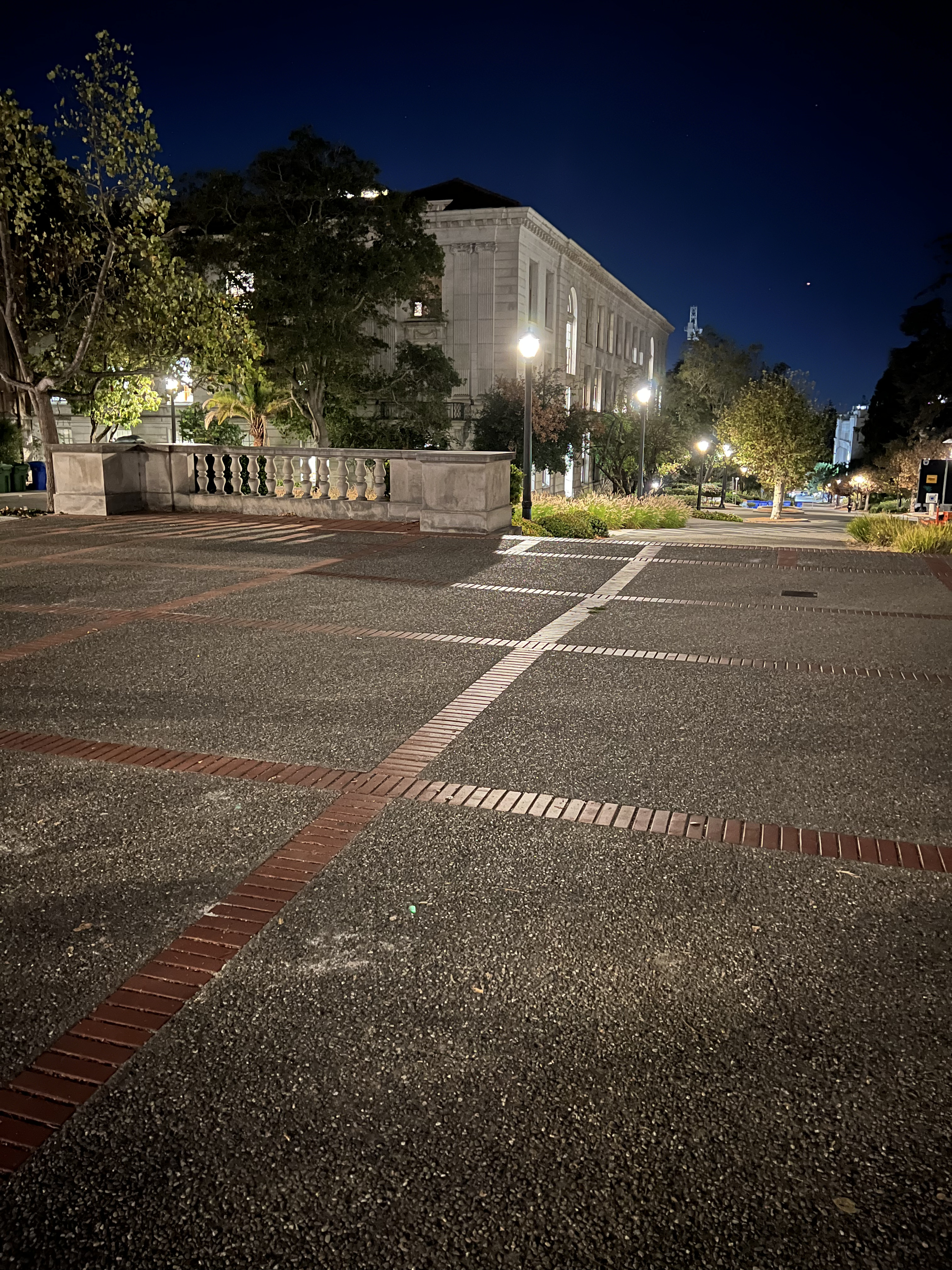
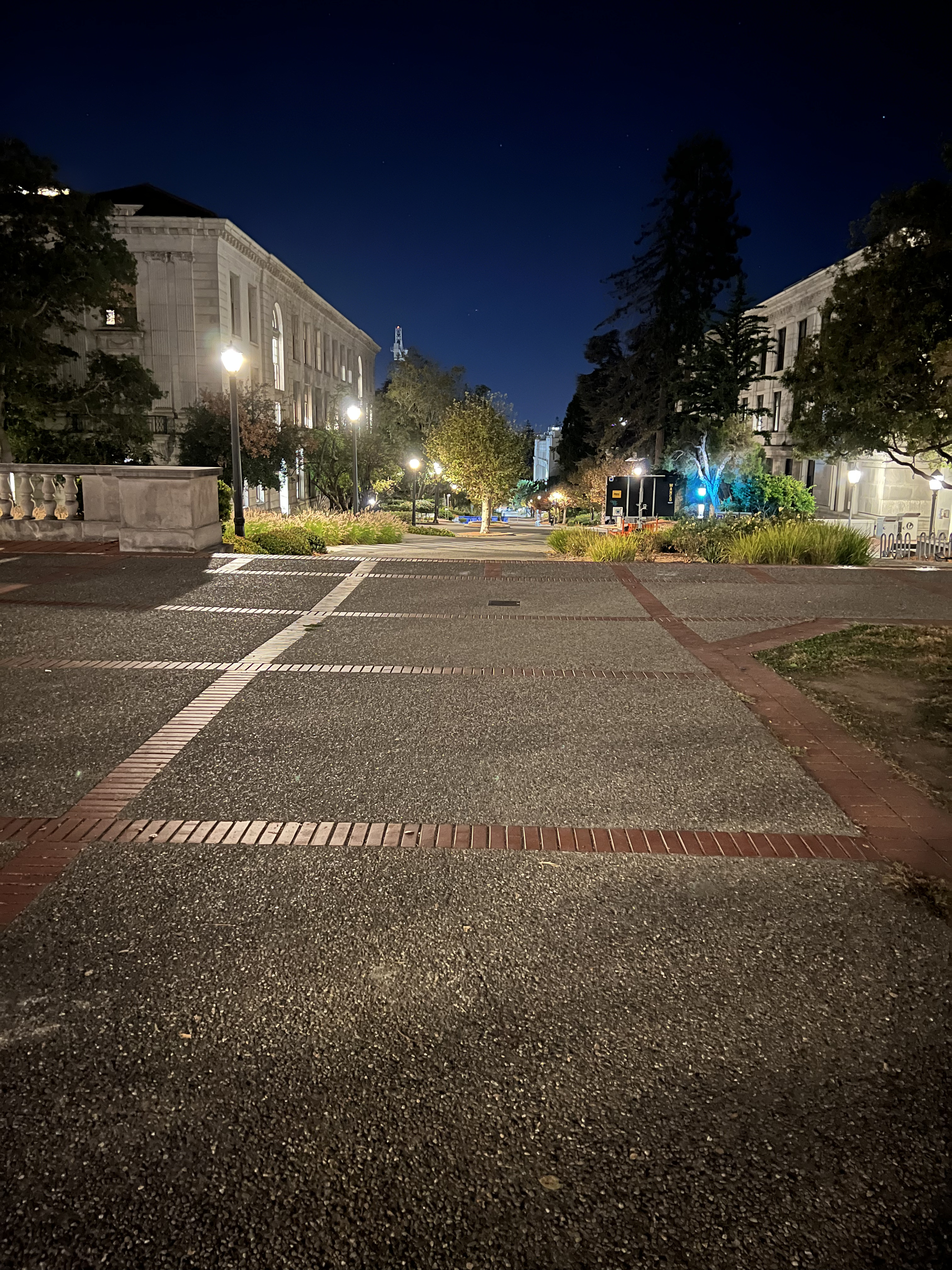
Below are the final results of the mosaicing process using the blending techniques described:
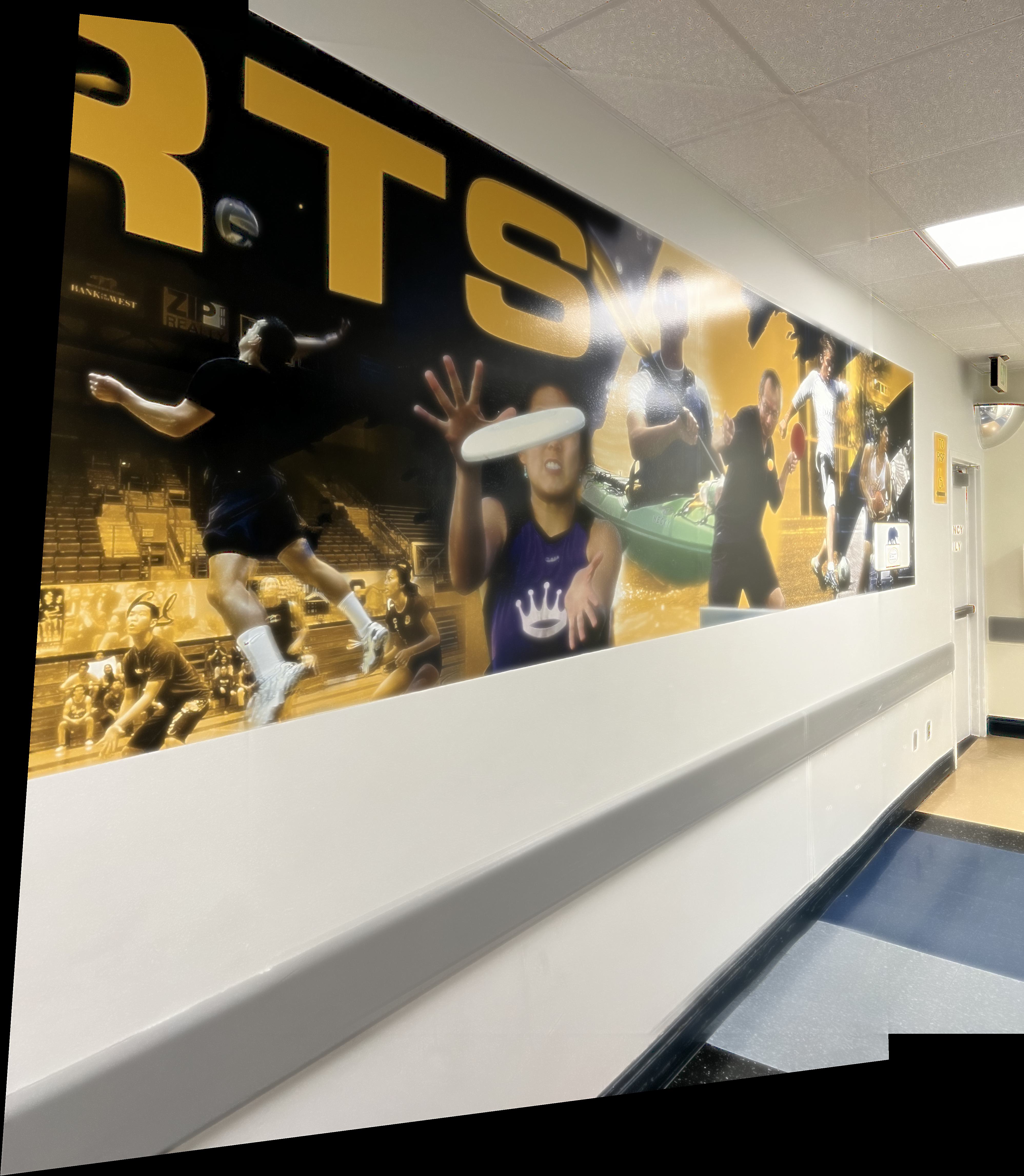
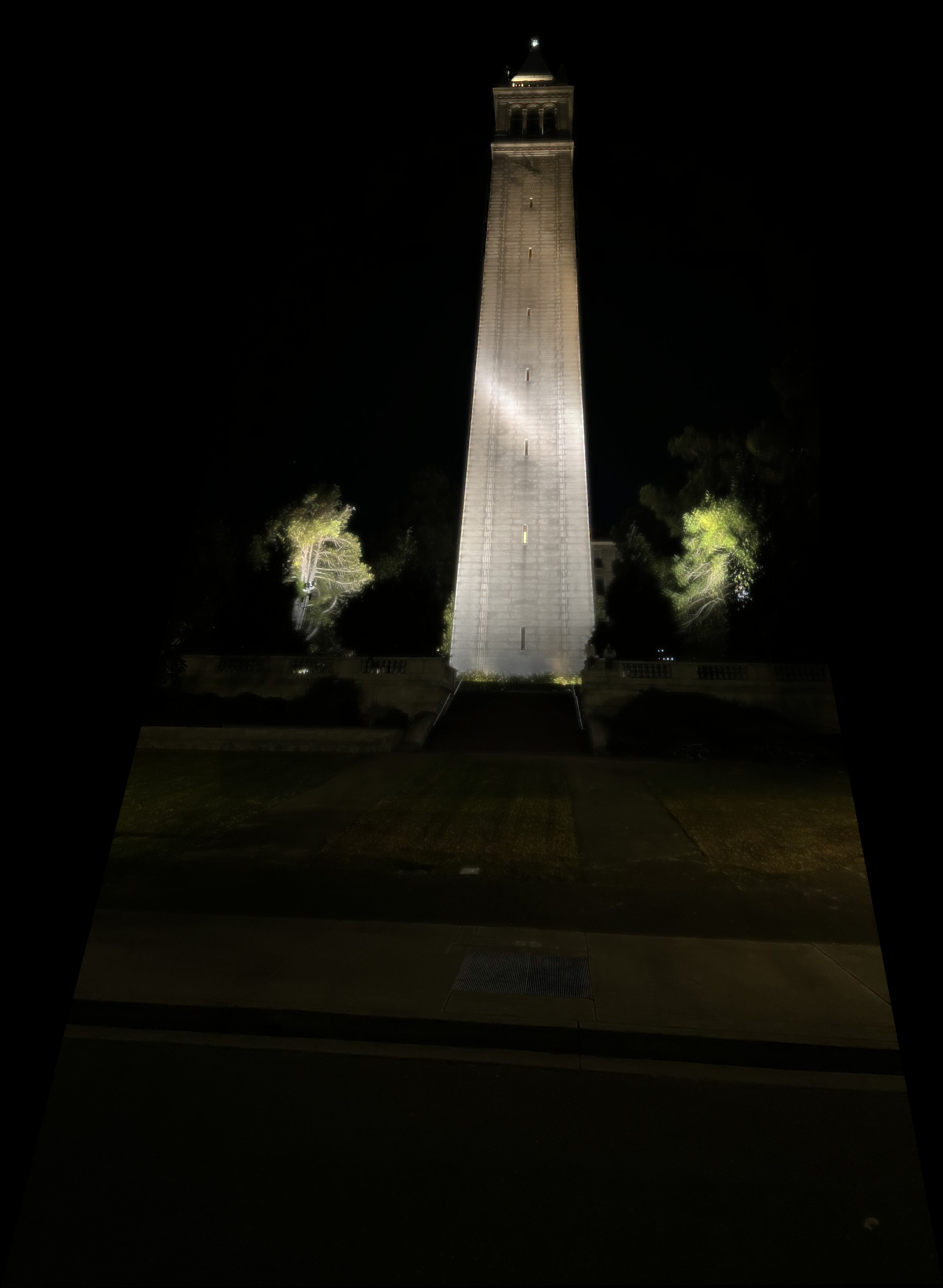
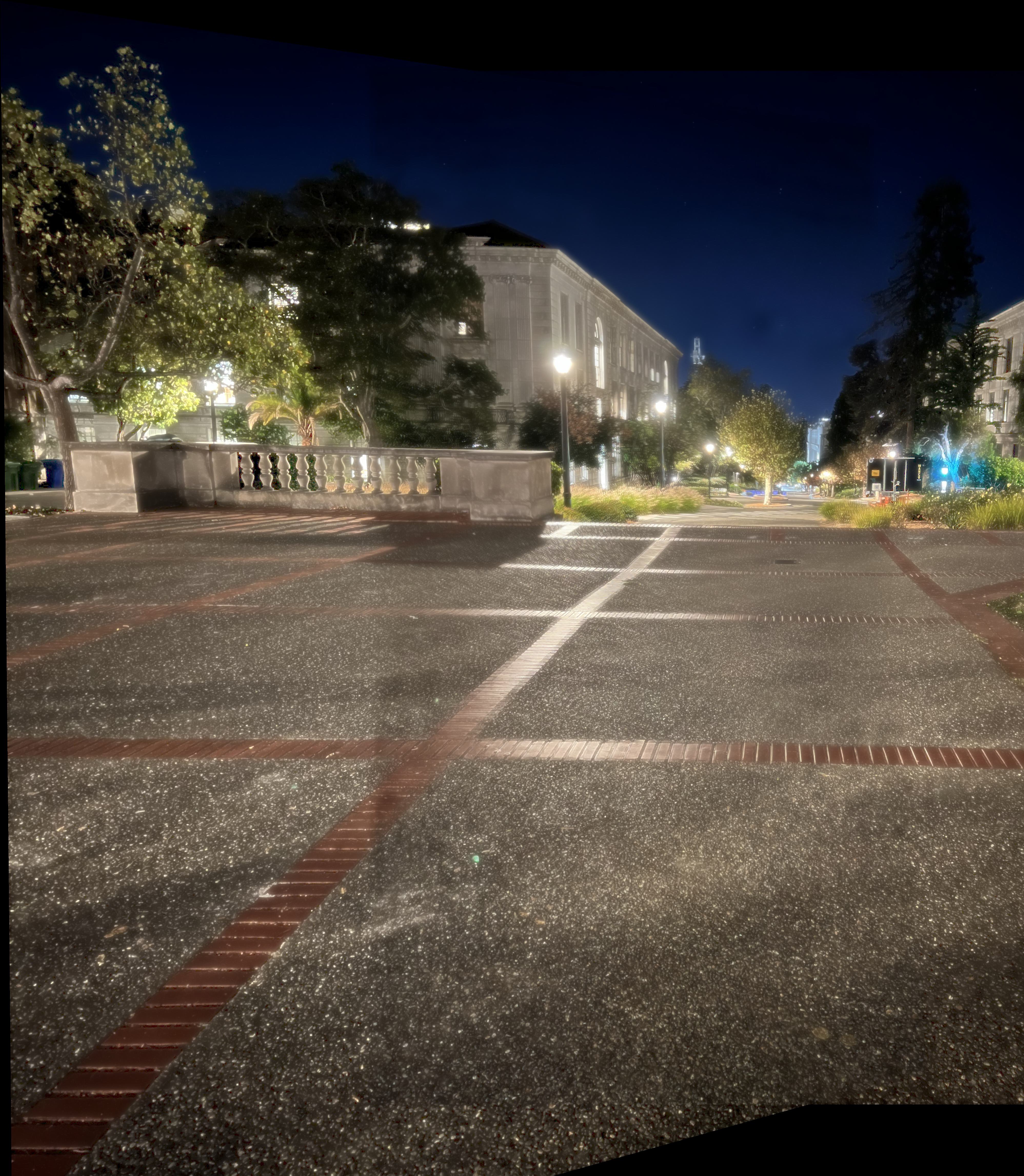
Directory containing final mosaic images:
It was exciting to see how basic linear algebra could lead to powerful methods like homography estimation, where a simple change of basis allows us to align images to a common plane. This not only enables seamless warping but also sets the stage for blending techniques that leverage low- and high-frequency components to create a cohesive, stunning final mosaic.
Here are the results of running the Harris corner detector on a sample image from just using the code provided in harris.py! Thank you! . The process transforms the black-and-white version of the image, assigning a "corner strength" value to each pixel. Pixels with a high corner strength compared to their immediate neighbors are identified as potential corner points. This produces many a lot and I mean a lot of pretty redundant (not much information obtained) candidates.
The image below shows the original image overlaid with Harris interest points detected in areas with high corner strength:

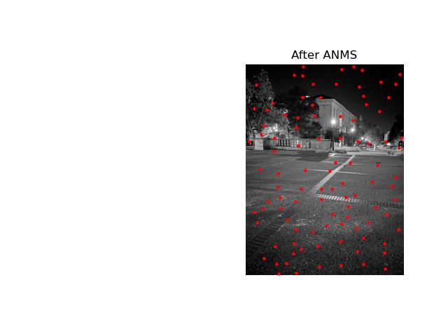
In the previous Harris corner detection, there were way too many candidate points to be meaningful. To address this, I followed instructions and simply applied the Adaptive Non-Maximal Suppression (ANMS) that was outlined in the following paper staff shared:https://inst.eecs.berkeley.edu/~cs180/fa24/hw/proj4/Papers/MOPS.pdf. This was done to filter out redundant keypoints, retaining only the strongest corners that are evenly spaced across the image. This made a big difference as it helped to reduce overlap and also ensured that selected points represent significant, well-distributed features at least that's the idea!
The images below show a comparison of detected corners before and after applying ANMS:

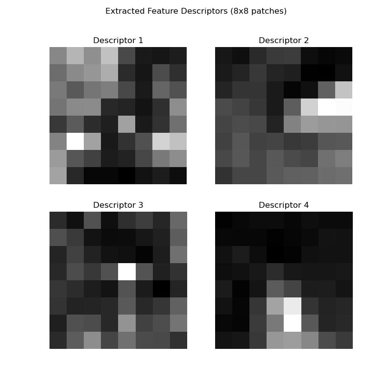
For feature descriptor extraction, I implemented axis-aligned 8x8 patches sampled from a larger 40x40 window around each keypoint. This approach was done to try and help ensure that we were able to get a sufficiently blurred descriptor for each feature point. I applied bias and gain normalization to standardize the descriptors for comparison. Note that rotation invariance and wavelet transforms were not applied in this implementation, focusing on the axis-aligned descriptor extraction.
Below are examples of extracted feature descriptors:
Once features are extracted from both images, the next step was to establish correspondences by matching features between them. For efficient matching, we use k-d trees to perform quick nearest-neighbor searches, where each feature in the first image is compared to potential matches in the second image. To ensure robust matches, a cross-check is applied, where a feature from the first image must have its best match in the second image, and vice versa. This bidirectional validation helps eliminate mismatches.
To further refine matches and minimize outliers, we apply a ratio test, inspired by Lowe’s method. By examining the ratio between the closest and second-closest matches for each feature, we can filter out ambiguous matches. Ideally, the closest match should be significantly stronger than the second-closest if it represents a true correspondence. This additional thresholding step enhances the reliability of our matching process.
The image below illustrates the results of feature matching on ANMS-selected points. Harris interest points are marked in blue, while ANMS-selected points are in red.
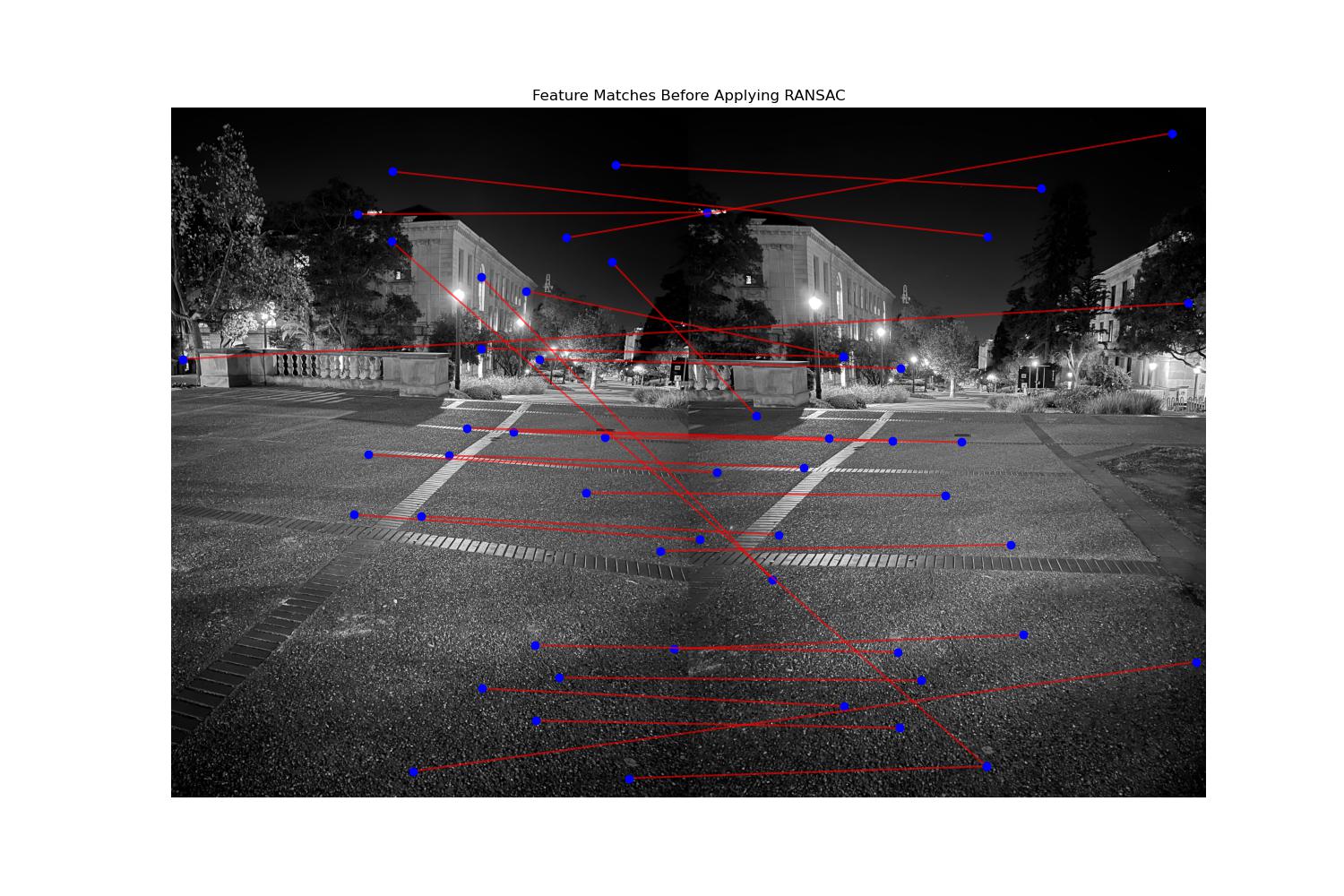
Yet even with Lowe's ratio test reducing outliers in feature matching, some incorrect correspondences still nonetheless remain, which can heavily influence the homography estimation calculation as a result of this "noise."" This is because the least-squares optimization is actually (without regularization) pretty sensitive to outliers, as it basically returns a safe "expectation" of the training data it can see. In fact there is some theory such as the James-Stein estimator that shows how shrinkage can help lead to a better general estimator when we have some conditions being met such as the data point being 3 or more parameters. a single mismatched pair can distort the result significantly. To address this, we use RANSAC (Random Sample Consensus) to improve robustness.
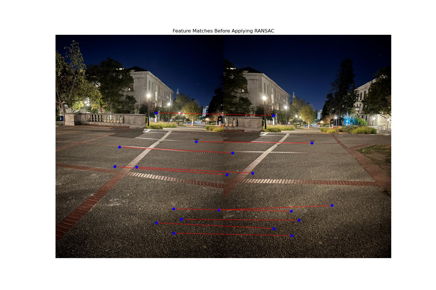
In RANSAC, we randomly sample four pairs of matched points and compute the homography based on these samples. We then evaluate how well this homography aligns other correspondences, counting the number of "inliers"—points that fit the homography within a defined error threshold. This process is repeated multiple times, and the homography with the highest number of inliers is selected as the best estimate. By prioritizing the consensus among inliers, RANSAC minimizes the impact of outliers and yields a more reliable homography.
The image below shows the effect of RANSAC on the matched features, with cross-checking disabled to highlight RANSAC’s impact on filtering outliers.
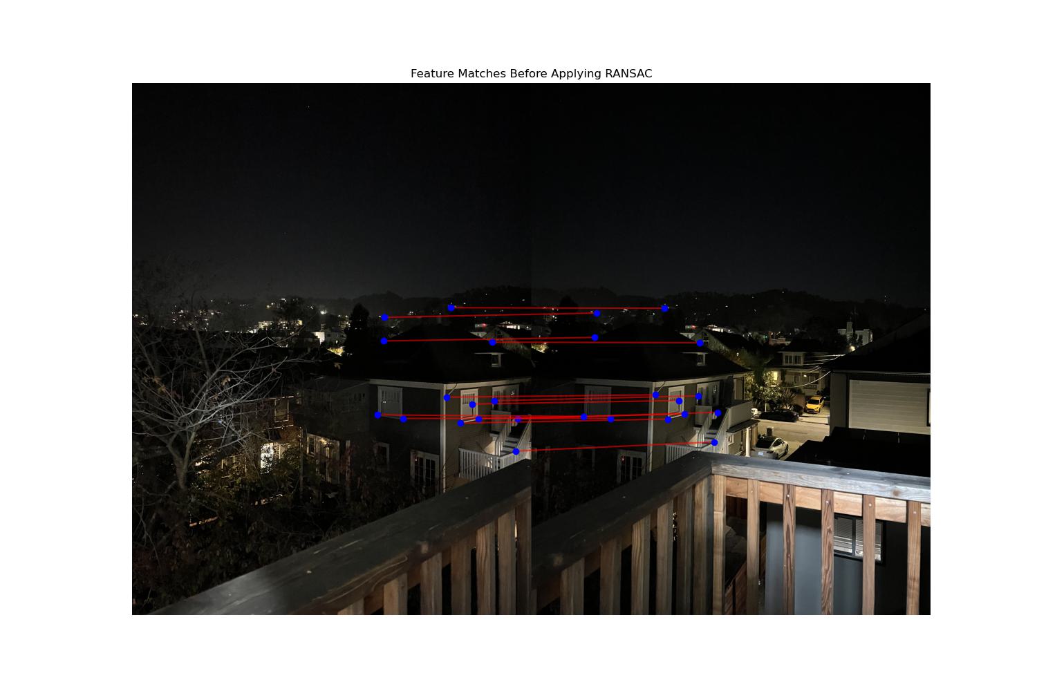
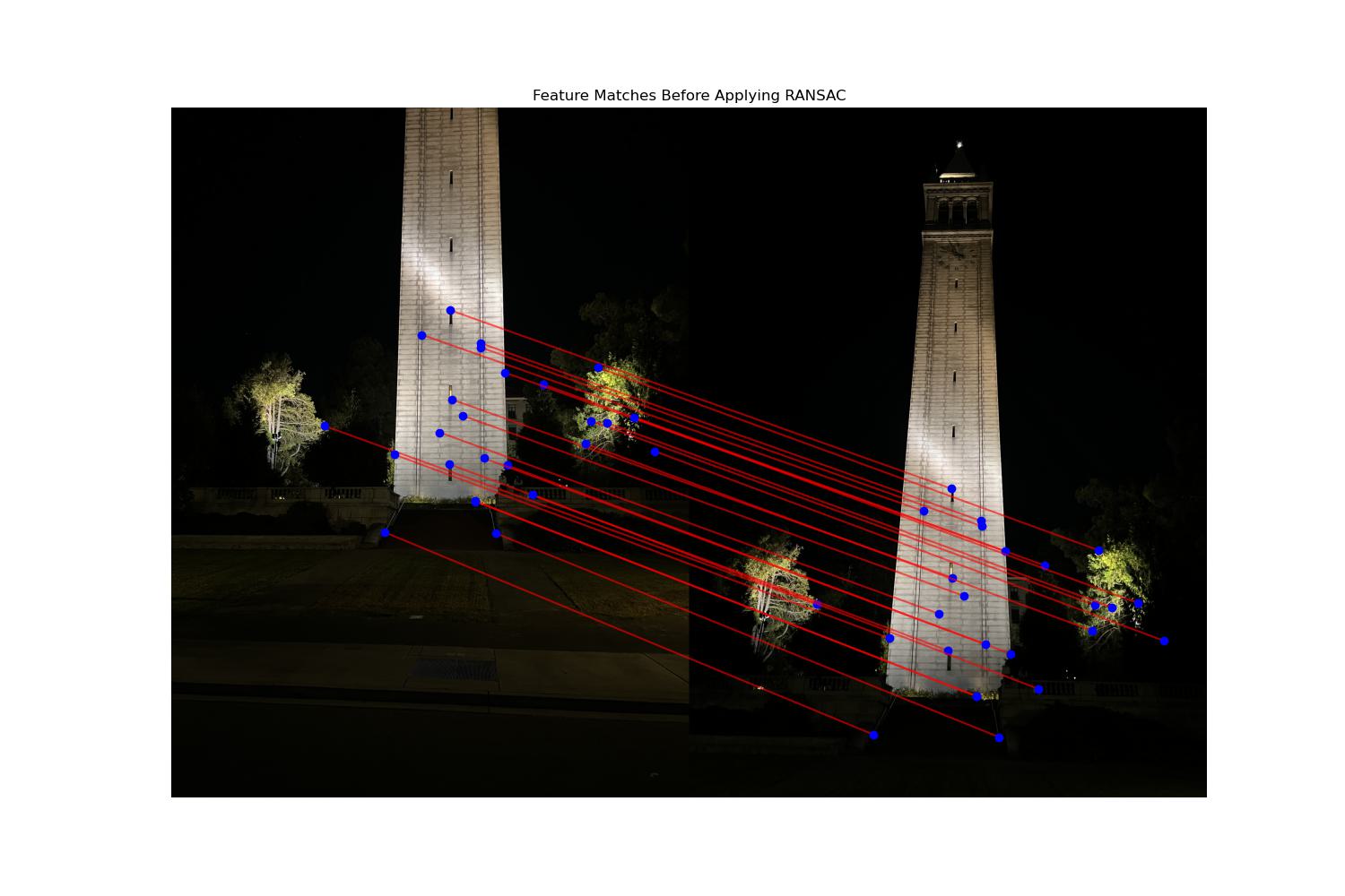
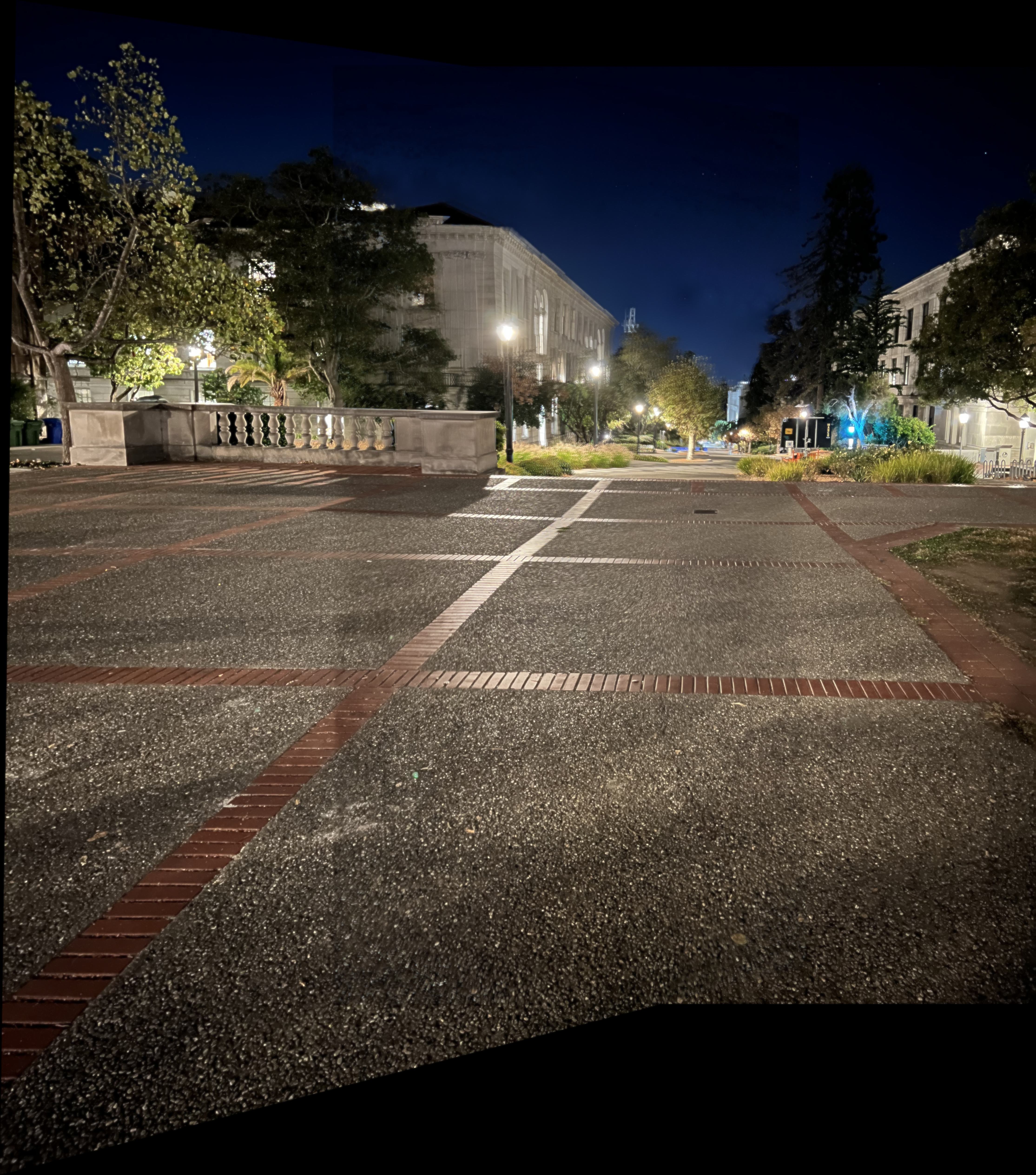
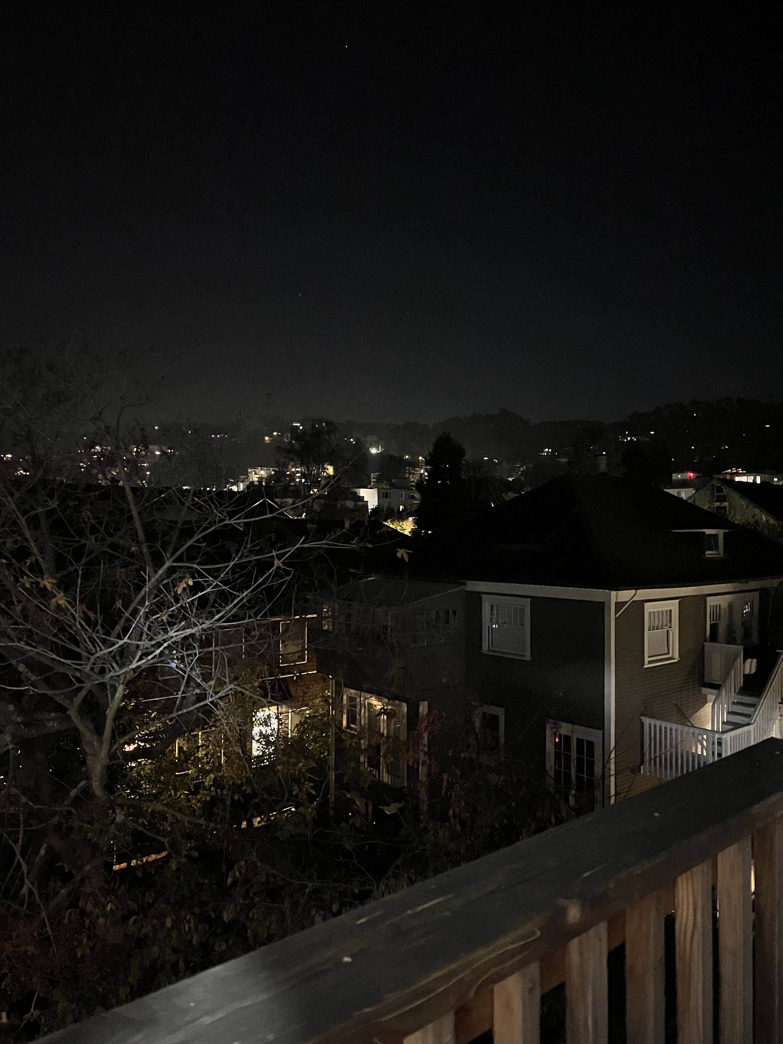
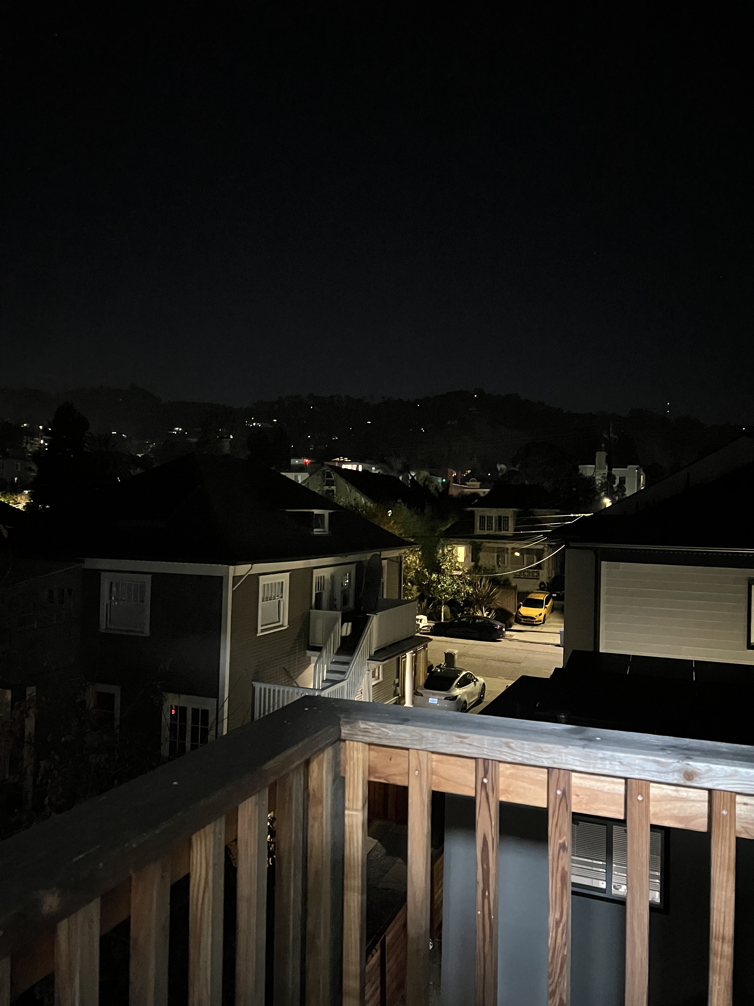
The following images demonstrate the outcome of the full feature detection, matching, and homography estimation pipeline. The final mosaic is built by blending transformed images using robust homographies from RANSAC, resulting in cohesive alignment.
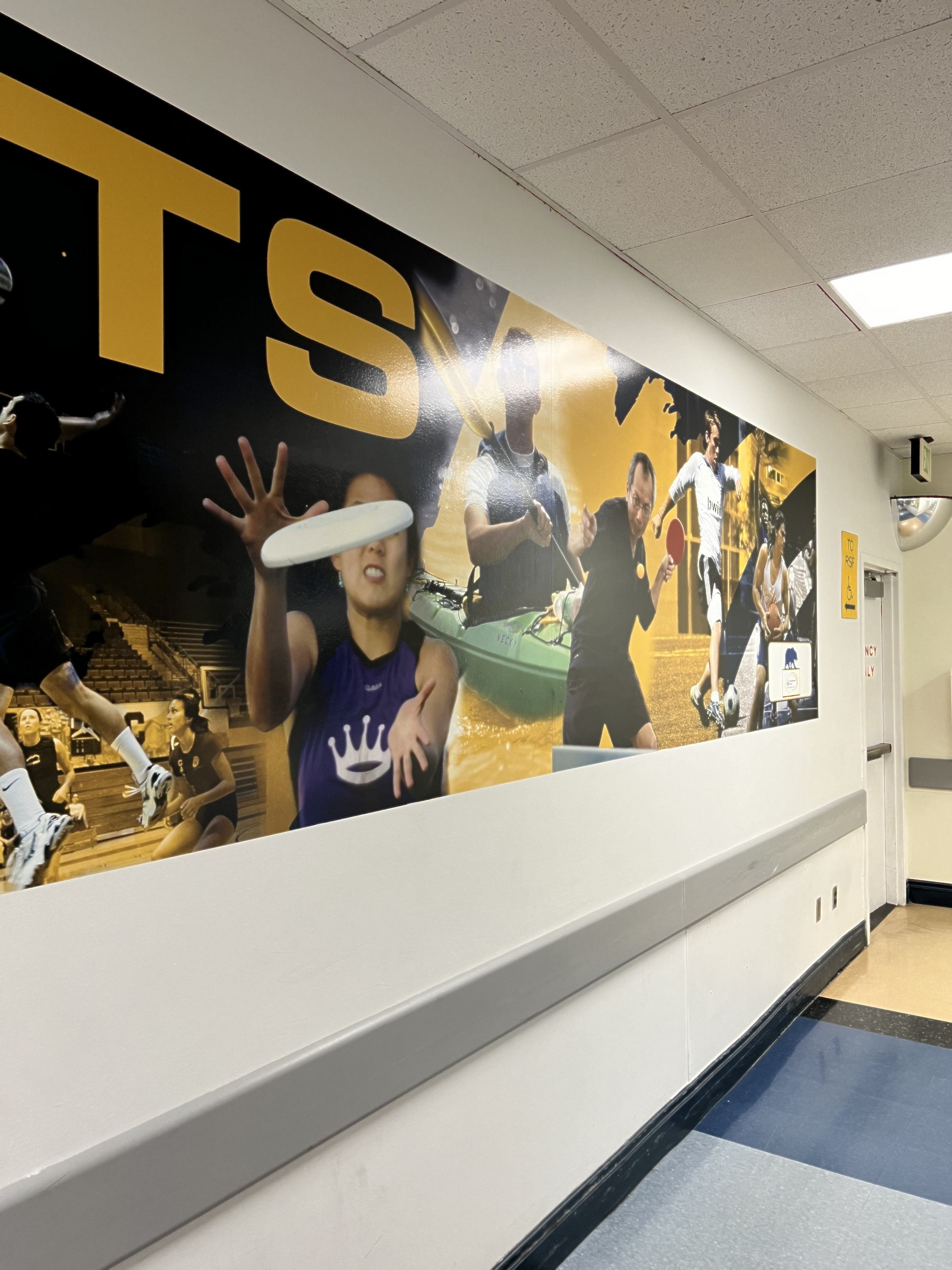

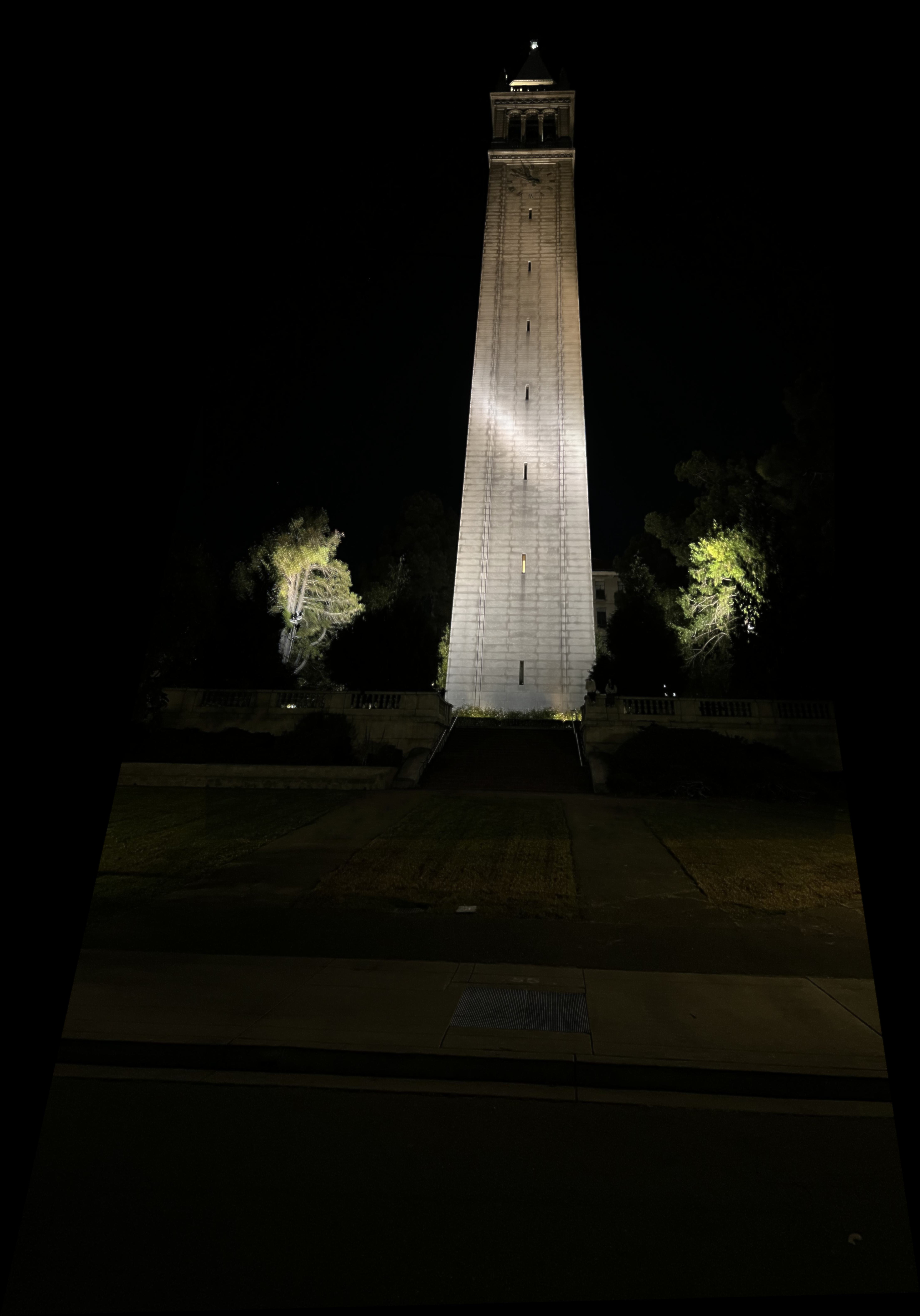


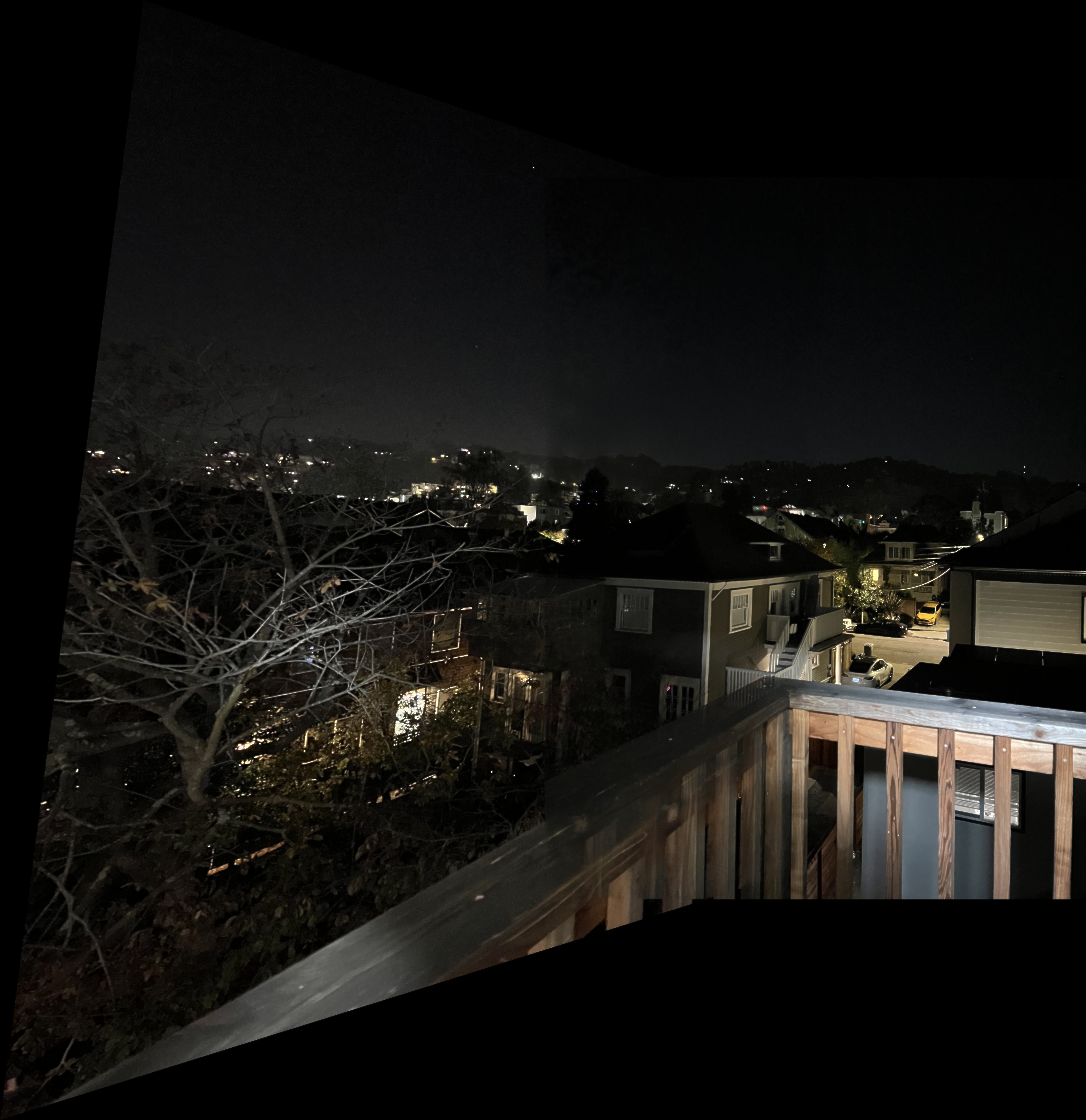
I was pleasantly surprised by how easy it is to construct panorama pictures. By the end of the project, I had fully automated the homography estimation, correspondence point detection, and implemented a seamless blending process that works with any images, all without requiring further input from me.